Background
Basic sorts such as bubble sort and insertion sort typically run in O(N2) time where N is the number of elements. This complexity makes these sorts exponentially slower as the size of the list being sorted increases.
Insertion Sort
In an insertion sort, we go from left to right, visiting each index in the list to be sorted starting with index 1 (assuming a zero-indexed list). Our goal is to insert each visited element in its proper position within the sub-list composed of all the elements to its left. If the visited element is greater than the element to its left, then due to the insertion sort invariant (described below) it is greater than all the elements to its left and does not need to be moved.
Description
Let’s call the currently selected index, the marker index, and the element at that index, the marker element.
Identify the insertion position of marker element: If the marker element is greater than the element to its left, then it is already in its proper position and we can advance to the next index in the list by incrementing the marker index by 1.
If not, the insertion position of the marker element is the position within the (by definition, sorted) sub-list formed by all elements to its left, such that all elements before the insertion position are less than or equal to the marker element, and all elements after the insertion position up to the marker index are greater than the marker element.
Note: If the marker element is smaller than all elements to its left, its insertion position will be the beginning of the list (index 0).
Insert marker element in the insertion position: Our next step is to move the marker element to the identified insertion position. We shift each element in the sub-list that is greater than the marker element (each element between the insertion position and the marker index) one position to the right, starting from the identified insertion position and moving up to the marker index. This creates an empty slot at the insertion position, into which we then place the marker element.
Now that the marker element is in its correct position in the sub list to the left of the marker index, we increment the marker index by 1. We repeat this until the marker index reaches the end of the list.
Invariant: In an insertion sort, the invariant (the condition that is always true during the execution of the sort) is that the sub-list formed by elements to the left of the right-traveling marker index is always fully sorted.
Efficiency Analysis
For N numbers, the marker moves to the right N-1 times and each time the marker is moved, there are as many comparisons as the current value of the right-moving marker index (1,2,3…N-1).
Hence the worst-case number of comparisons in one full run of the insertion sort is ∑(N-1) which is N(N-1)/2.
However on average, assuming uniformly random data, for each marker position at index n, we perform about n/2 comparisons since the insertion point is equally likely to be anywhere in the sorted sub-list to the left of the marker position, and hence the total number of comparisons for the average full run of the insertion sort is half of the worst case, or 1/2*∑(N-1) which is N(N-1)/4.
The total number of element shifts (when the element is moved one place to the right to accommodate the space made for the marker element) is approximately the same as the number of comparisons since each comparison that leads to insertion requires shifting one element to the right.
Thus the total number of operations – comparisons plus right shifts – on an average insertion sort is 2 * N(N-1)/4, which is N(N-1)/2.
Insertion Sort vs Bubble Sort complexity
While the insertion sort runs in O(N2) time, it still runs about twice as fast as the bubble sort since the number of comparisons and element copies (to their adjacent position) are on average about half the number of element comparisons and swaps that happen in the bubble sort.
Also, a copy operation (the basic repeated operation in an insertion sort) is less time consuming than a swap operation (the basic repeated operation in a bubble sort).
In a best case scenario, when the array is already sorted, no shifts are required and insertion sort completes in linear time: O(N). In the worst case scenario, if the data is inversely sorted, each marker must be inserted at position 0, and the insertion sort has to do n comparisons and shifts for a marker value of n, rather than the average n/2, and hence the insertion sort degenerates to O(N2) time, which is the efficiency of the bubble sort.
Shell Sort
Shell Sort is a faster form of insertion sort.
The Shell Sort is considered one of the easier sorts to implement. The shell sort is a series of insertion sorts performed on sub-lists of the list to be sorted.
The basic idea in Shell Sort is to perform insertion sort on sub-lists comprised of elements whose index is separated by a gap value, for a series of gap values. By starting with large gap values, Shell Sort allows smaller elements that are out of place to move large distances across the list to be closer to their proper ordered position without shifting any intermediate elements. With each iteration, the gap is reduced, and the list becomes progressively more ordered.
In the final iteration, when the gap is reduced to 1, Shell Sort effectively performs a standard insertion sort—but by then, the list is already nearly sorted, so very little work remains to be done.
Gap Sequence
Before we go further into the shell sort, we need to understand the concept of the gap sequence. This is simply a sequence of numbers where we start at a certain number, and on each pass, we apply a gap formula to the current sequence value, to get the next sequence value. The gap formula could be something as simple as dividing the current gap value by 2. The only requirement is that the sequence should have the value 1 within it. The current value of the gap sequence is called the gap value. So the requirement is that one of the gap values generated by the gap sequence has to be 1. It doesn’t take a lot of intuition to determine why the number 1 is so important. A gap value of 1 signifies a normal and full insertion sort. Let us hold that thought for later.
Gap Value constraints and properties
- The start value of the current gap value (h) obviously has to be the less than the size of the list of elements being sorted.
- The final gap value must be 1 to ensure that the array is fully sorted by running an insertion sort on the last iteration.
- Gaps should be non-repeating and typically strictly decreasing.
- Gaps should ideally be coprime with each other or vary non-trivially to break patterns.
- They should allow for both coarse and fine comparisons (start large, shrink gradually).
- The rate of decay matters: too steep → not enough work early; too slow → redundant passes.
Shell Sort’s insertion sort
- In a regular insertion sort, starting with the 2nd element, we visit each element all the way to the last element of the list, and insert the visited element in its appropriate position in the sub-list that is composed of itself and all the elements to its left. The (usually unstated) condition here is that the gap between indexes of adjacent elements of a sub-list in the regular insertion sort is 1. This is why the sub-list is composed of all the elements to the left of the currently selected element in addition to the selected element itself.
- In the shell sort, an insertion sort is run for each gap value generated by the gap sequence starting with a start gap value all the way down to a final gap value of 1. Remember that the start gap value has to be smaller than the size of the list of elements to be sorted.
- In each iteration of the generalized insertion sort that is run by the shell sort, given the current gap value of h, we visit each element starting with the hth element of the list all the way to the last element of the list, and insert the currently visited element in its appropriate position in the sub-list that is composed of itself and all the elements to its left (just like we do in insertion sort) whose indexes are separated from the currently visited element by a positive multiple of h (in standard insertion sort, h = 1). The distance between any two adjacent elements of this sub list is always h.
Eg: If the currently selected element has an index i and current gap value is h, then the sub-list will be {A[i], A[i-h], A[i-2h], A[i-3h],A[i-4h]….A[i-kh]} such that i-kh >= 0 and k is a positive integer.
- Note: If the currently selected element is already the greatest element in the sub-list, then it does not need to be moved.
- In mathematical terms, given 2 elements of the sub-list with indexes i1 and i2, then |i1-i2| = kh where k is a positive integer. Regular insertion sort can be seen as a special case of the generalized insertion sort that is run by the shell sort where the gap value is 1 (h = 1).
- Reverse direction sub-lists: A point of note is that in each iteration of the shell sort’s insertion sort which runs for a specific gap value h, the sub-lists are formed in the reverse direction starting with an end index i such that h ≤ i ≤ n (i ranges from h to the end of the list) where n is the last index of the list being sorted
- When the current gap value reaches 1 (h = 1) on the last iteration of the shell sort, in effect a standard insertion sort is run over the list.
Alternate visualization of Sub-list selection – forward direction sub-lists.
Another helpful way to form a mental picture of the sub-lists formed for each iteration of the insertion sort run within the shell sort is to visualize them as forward direction sub-lists. Here i is the start index of each sub-list and 0 ≤ i ≤ h-1. (i ranges from 0 to h-1). h is the current gap value.
Eg: For a gap value h and a sub-list start index value of i, the sub-list will be: {A[i], A[i+h], A[i+2h], A[i+3h],A[i+4h]….A[i+kh]} such that i+kh < N where N is the size of the list and k is a positive integer. In other words, i + kh cannot exceed the size of the list.
Other Points
With every iteration of the shell sort, the previous value in the gap sequence becomes the current gap value (h), continuing until h = 1, at which point a final insertion sort is performed on the full list. The gap value shrinks with each iteration, until it finally reaches the value of 1.
At the end of each iteration of the shell sort for a gap value h, the list is said to be h-sorted.
After each iteration, the list becomes progressively more sorted, making subsequent passes more efficient.
By the time the current gap value reaches the number 1, the multiple sub-list insertion sorts that have occurred previously ensure that the list is partially or almost fully sorted.
Gap Sequence Generator Function
As with all sequences in math, the gap sequence is generated by a generator function. There is a whole range of functions that have been proposed. A more detailed discussion regarding the sequence generator functions can be found here.
Key Qualities of a good Gap Sequence Generator Function
A primary criterion that determines a good gap generator function is that the list should be nearly sorted by the time the sequence reaches 1. The sequence generated by the function must have the number 1 within it.
Gaps should be non-repeating and ideally co-prime with each other or at least not share many factors between themselves, or you risk missing out on sorting between some indexes until very late. The gaps are not required to be relatively prime though.
Optimal number of gaps to balance coverage and redundancy: The number of gaps generated by the sequence should be enough to allow for meaningful element comparisons across the list, but not so many that multiple iterations of sub-list insertion sorts are run by the shell sort with little effect on the disorder within the list, thereby wasting time.
The gaps should start large, and shrink gradually. The rate of shrinking of the gap matters – too steep -> not enough work early; too slow -> many redundant passes. Explained below.
Early gaps should be large..
The earlier gaps in the sequence should be large enough to allow elements to move large distances across the list (and therefore closer to their correct position within the list), thereby allowing smaller elements to move towards the beginning of the list and larger elements towards the end.
… but not too large relative to the size of the list
Too large gaps will create sub lists with very few elements. This leads to computationally intensive iterations that perform too few meaningful swaps because the gap is too large and elements too few to catch most inversions (element exchanges) which barely reorders the array, and leaves most of the sorting work for later iterations. This is not optimal and will tend the sort time complexity towards that of the standard insertion sort.
If the early gaps are too large and the gaps shrink too fast towards 1:
We end up fixing only a few far apart inversions and missing opportunities to fix mid-range disorder in the early iterations. This leaves a lot of work for the few later passes, and essentially the last pass (which is the insertion sort) ends up doing most of the work.
If the early gaps are too large and the gaps shrink too slowly towards 1:
- Early on, you do low value iterations which leave much of the disorder in place and unhandled.
- Overall you do too many passes, especially near the end when gaps are small and gap size tends towards 1.
- You still pay the cost of traversing and sorting subarrays that aren’t very disordered.
- The total runtime balloons because you’re doing too much shallow cleanup before the deep cleaning starts.
If the early gaps are too small, shell sort begins to resemble the plain insertion sort, negating the advantages of the Shell Sort over the insertion sort. Also, smaller early gaps mean you are missing out on the global repositioning efforts of the Shell Sort. The Shell Sort’s key advantage is that it lets elements jump long distances early, quickly reducing global disorder.
- Far-apart inversions remain untouched until very late.
- You need more swaps and comparisons in later passes.
- The final insertion-sort-like phase ends up doing all the heavy lifting, affecting performance.
| Property | Description |
| Starts with moderately large gaps relative to the size of the list being sorted. | Ensures distant swaps and rapid early progress |
| Shrinks geometrically or using optimized formulas | Avoids excessive passes, or too few early passes and leaving most of the work for later passes. |
| Avoids small early gaps | Prevents redundant early work, and reduces global disorder. Reducing global disorder is a primary advantage of the Shell Sort. |
| Ends with a gap of 1 | Guarantees final pass is a true insertion sort, which is a mandatory requirement for a successful Shell Sort. |
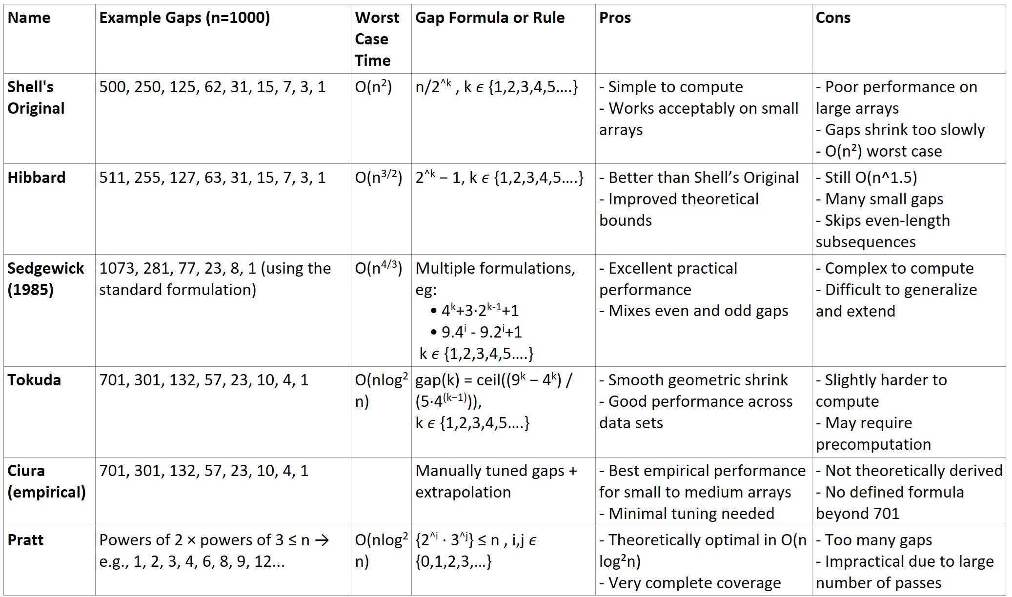
Example Gap Sequences and their pros and cons
Shell Sort Algorithm
Description
Shell sort is essentially a set of insertion sorts run for a set of diminishing gaps determined by the gap generator function that goes from a start gap value h down to 1 where h < N (size of the list).This start gap value must be less than the size of the list.
For each gap value h, exactly h sub-lists are identified within the list and the list is insertion sorted in-place for that gap value using the identified sub-lists. One sub-list for each value of i where h ≤ i ≤ n. n is the last index of the list.
Let us call i as the marker index. Each sub-list is formed by grouping together elements within the list whose index value idx = (marker index i)-(k*h) where i = (h, h+1, h+2, h+3, h+4…..n) in other words, h ≤ i ≤ n. h is the current gap value, k is a whole number. k ϵ {0,1,2,3,4….} and n is the last index of the list.
For example: Given a list to be sorted A and i = (h, h+1, h+2, h+3. h+4…) then the first sub-list would be {A[h], A[h-h]} or {A[h], A[0]}, the second sub-list would be {A[h+1], A[h+1-h]} or {A[h+1], A[1]} (will also include A[0] if h=1) third sub list would be {A[h+2], A[h+2 -h]} or {A[h+2], A[2]} (will also include A[1] and A[0] if h=1) and so on.
All h sub-lists identified for a gap value are sorted in-place by moving elements within them to their correct position within the sub-list relative to the other elements of the sub-list. At the end of one iteration for a gap value h, the list is said to be h-sorted.
Once h has reached a value of 1, the list has been h-sorted for a number of gap values, and ideally should be close to fully sorted. At this point because h = 1, we are essentially running a regular insertion sort on the nearly sorted list. At the end of this iteration, the list has been fully sorted.
Implementation Steps:
- Similar to insertion sort, we start with a value that we will call the marker index i, where starting value of i = h, the current gap value.
- The marker index thus moves from h to n for each gap value – each value of h.
- Given the current value of the marker index i and current gap value of h, we compare A[i] with all the elements in its sub-list (A[i-h], A[i-2h], A[i-3h]….) such that i-kh >= 0 and k is a positive integer. We then increment the marker index by 1 and repeat this step until the marker index reaches the end of the list.
- We repeat the above step for each decreasing gap value all the way down to a gap value of 1.
- At the end of the iteration for a specific gap value h, the overall list is said to be h-sorted where h is the gap’s current value.
- This process is repeated until the gap value reaches 1 (h = 1), which means that the final iteration (with a gap size of 1) is a regular insertion sort.
- Note that all of this is performed in-place on the list being sorted, which means that no additional space is allocated nor sub-lists created in memory.
Code Examples
Below is an example of what the actual code that implements the above algorithm looks like:
Python
 # Generate initial Knuth gap
    gap = 1
    while gap < n // 3:
        gap = 3 * gap + 1  # 1, 4, 13, 40, ...

    while gap > 0:
        for i in range(gap, n):
            temp = arr[i]
            j = i
            while j >= gap and arr[j - gap] > temp:
                arr[j] = arr[j - gap]
                j -= gap
            arr[j] = temp

        gap //= 3

# Example usage
arr = [37, 22, 0, -5, 19, 8, 45, 3]
shell_sort(arr)
print(arr)

def shell_sort(arr):
    n = len(arr)
Java
public class ShellSort {
    public static void shellSort(int[] arr) {
        int n = arr.length;

        // Generate initial Knuth gap: 1, 4, 13, 40, 121, ...
        int gap = 1;
        while (gap < n / 3) {
            gap = 3 * gap + 1;
        }

        // Perform Shell sort
        while (gap > 0) {
            for (int i = gap; i < n; i++) {
                int temp = arr[i];
                int j = i;

                while (j >= gap && arr[j - gap] > temp) {
                    arr[j] = arr[j - gap];
                    j -= gap;
                }

                arr[j] = temp;
            }

            gap /= 3;
        }
    }

    public static void main(String[] args) {
        int[] arr = {37, 22, 0, -5, 19, 8, 45, 3};
        shellSort(arr);
        for (int num : arr) {
            System.out.print(num + " ");
        }
    }
}
Time Complexity
Shell sort is in many cases an improvement on insertion sort, which has a time complexity of O(N2). Shell sort complexity can range from best case: O(NlogN) to worst case: O(N2). Please see section on Gap Generator Functions to see the range of possible time complexities for the Shell Sort.
Additional Resources
See big O notation for a refresher on time complexity.
Leave a Reply